This post is on one of the nasty prerequisites for all data professionals: "Understanding Dirty Data and How to Clean it Up". Sometimes called "bad data" or alternatively the quest for "tidy data". Most 'relational data' uses the row and column format as you are familiar with in a spreadsheet. Ideally, all data would be arranged neatly in such a format. Let us take a look at such data from R's data editor window. You can click on these pictures to see them in the blogger slide viewer:

So this data is part of the EPA 2013 fuel economy ratings. You can see the steps I took to get this data into the data editor here (click to enlarge):

All well so far. Now let us try some data analysis! Let us say, for example, that you want a list of all vehicles whose combined MPG is 45 or more. The following syntax should work just fine, if your data was "clean":
> subset(EPADelim, Cmb.MPG >= 45 , select = c(Model,Cmb.MPG))
[1] Model Cmb.MPG
<0 rows> (or 0-length row.names)
Warning message:
In Ops.factor(Cmb.MPG, 45) : >= not meaningful for factors
However, a warning message is returned. So let us take a look at 'Cmb.MPG'. Right away, we see some problems. Many of the data fields are marked "N/A". By default, R ignores these entries. More troublesome for those of us who would like to do numeric comparisons with the subset function is "factor" data fields such as "16/24". These fields can not be subject to numeric comparison by R.:

To understand data a little better, let us discuss (briefly) 'datatypes' in R. R has a number of important classes of data. You can use the 'class()' function on any object in R to uncover the class type. For example:
> class(1)
[1] "numeric"
> class("char")
[1] "character"
> class(1:10)
[1] "integer"
> class(2303456L)
[1] "integer"
> class(df)
[1] "data.frame"
> class(get.c)
[1] "function"
The class of the data can be changed with the 'as.[class]' function:
> class(EPADelim$City.MPG)
[1] "factor"
> class(as.numeric(EPADelim$City.MPG))
[1] "numeric"> (as.numeric(EPADelim$City.MPG))
[1] 52 52 52 40 40 38 38 29 29 32....
> class(as.vector(EPADelim$City.MPG))
[1] "character"
> as.vector(EPADelim$City.MPG)[1:10]
[1] "39" "39" "39" "24" "24" "22" "22" "16" "16" "19"
So let us try our subset() function once again, converting 'Cmb.MPG' datatype on the fly:
> subset(EPADelim,as.numeric(Cmb.MPG) >= 45,select = c(Model,Cmb.MPG))
Model Cmb.MPG
1 ACURA ILX 38
2 ACURA ILX 38
3 ACURA ILX 38
4 ACURA ILX 28
5 ACURA ILX 28
...
hmmm.... that isn't quite right. This data set has to be cleaned. R has an entire series of functions designed to help you automate such data "reshaping" including (but not limited to):
- strssplit()
- sapply()
- sub()
- gsub()
- cut()
- cut2()
- merge()
- melt()
- sort()
- order()
- head()
- tail()
I won't discuss these functions in this post. (See note at bottom for some tutorial links.) However, If you have some knowledge of a database language utility like 'gawk 4.0', you can use the following syntax to understand just how much data needs to be 'cleaned' in column 15. For example , sorted count of all data that contains the "/" in column 15 ('Cmb.MPG') shows:
$ gawk -F"\t" '{print $15}' all_alpha_13.txt | sort -nr | uniq -c | sort -k1 -nr | grep "/"
165 N/A
22 10/14
17 13/17
11 17/23
11 16/22
9 14/19
9 11/15
8 12/16
7 11/14
6 16/24
5 14/20
4 9/12
4 43/100
4 16/21
4 13/18
4 10/13
....
However, a much easier, but time consumptive, way to do this is by editing the data in a spreadsheet or R's data editor. The changes you makes in R's data editor take place immediately and irrevocably. You can see the approach I take to cleaning up data in the spreadsheet screenshot below. I simply split up the 'Cmb.MPG' into two numeric columns: 'Cmb.hi.MPG' and 'Cmb.lo.MPG'. :

> subset(EPASplit15,as.numeric(Cmb.hi.MPG) > 45 ,select = c(Model,Cmb.hi.MPG))
....
164 RAM 3500 N/A
165 RAM 3500 N/A
166 TESLA Model S 95
173 TESLA Model S 89
174 TOYOTA RAV4 EV 76
175 CODA Coda 73
176 CODA Coda 73
177 TOYOTA Prius Plug-in Hybrid 95
178 TOYOTA Prius Plug-in Hybrid 95
179 TOYOTA Prius 50
180 TOYOTA Prius 50
181 TOYOTA Prius c 50
182 TOYOTA Prius c 50
183 FORD C-MAX Hybrid 47
184 FORD Fusion Hybrid 47
213 CHEVROLET Volt 98
214 CHEVROLET Volt 98
215 CHEVROLET Volt 98
A better command line 'fix' for this would be:
EPASplit15$Cmb.hi.MPG <- as.numeric(EPASplit15$Cmb.hi.MPG) As a last resort we call up the data editor for EPASplit15 ('fix(EPASplit15)') and by clicking on the top column of the 'Cmb.hi.MPG' and 'Cmb.lo.MPG' convert them to numeric columns:

Now our subset() function works as desired:
> subset(EPASplit15,(Cmb.hi.MPG) > 45 ,select = c(Model,Cmb.hi.MPG))
Model Cmb.hi.MPG
166 TESLA Model S 95
173 TESLA Model S 89
174 TOYOTA RAV4 EV 76
175 CODA Coda 73
176 CODA Coda 73
177 TOYOTA Prius Plug-in Hybrid 95
178 TOYOTA Prius Plug-in Hybrid 95
179 TOYOTA Prius 50
180 TOYOTA Prius 50
181 TOYOTA Prius c 50
182 TOYOTA Prius c 50
183 FORD C-MAX Hybrid 47
184 FORD Fusion Hybrid 47
188 FORD C-MAX PHEV 100
189 FORD C-MAX PHEV 100
190 FORD Fusion PHEV 100
191 FORD Fusion PHEV 100
213 CHEVROLET Volt 98
214 CHEVROLET Volt 98
215 CHEVROLET Volt 98
2128 SCION iQ EV 121
2129 SCION iQ EV 121
2147 HONDA Fit 118
2148 HONDA Fit 118
2149 FIAT 500e 116
2150 FIAT 500e 116
2151 NISSAN Leaf 116
2152 NISSAN Leaf 116
2153 MITSUBISHI i-MiEV 112
2154 MITSUBISHI i-MiEV 112
2174 SMART ForTwo Cabriolet 107
2175 SMART ForTwo Cabriolet 107
2176 SMART ForTwo Coupe 107
2177 SMART ForTwo Coupe 107
2178 FORD Focus BEV 105
2179 FORD Focus BEV 105
Update 03/02/2013:
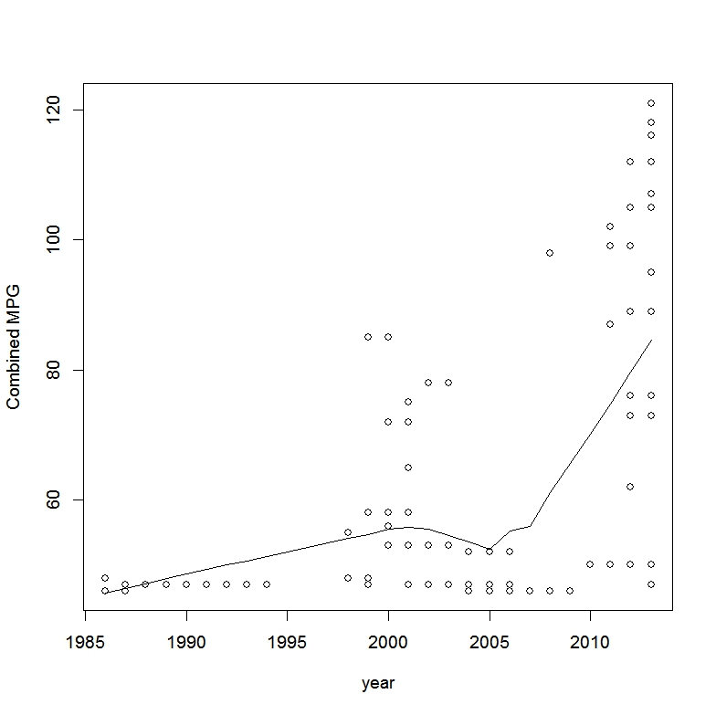
Originally, I missed a developer download page that had cleaner (and more detailed) fuel economy data. The chart below shows us how many high mileage vehicles are now appearing on the market.
# Download:
# http://www.fueleconomy.gov/feg/epadata/vehicles.csv.zip
# Unzip vehicles.csv to your working directory
AllVehicles <- read.csv("vehicles.csv")
AllVehicles$comb08 <- as.numeric(AllVehicles$comb08)
GTR45 <- data.frame(subset(AllVehicles, comb08 > 45, select = c(model,make,year,comb08,comb08U,combA08,combA08U,combE)))
# If necessary install (plyr) package.
# See dataframe sorting discussion at
# http://stackoverflow.com/questions/1296646/how-to-sort-a-dataframe-by-columns-in-r/6871968#6871968
# Sort by year then combined fuel mileage
# for other alternatives see[1,2]
library(plyr)
arrange(GTR45,(year),comb08)
SortYearGTR45 <- arrange(GTR45,(year),comb08)
plot(SortYearGTR45$year,SortYearGTR45$comb08,type="p")

Another method of sorting by dataframe with statistical smoothing:
GTR45.MPG.Year.Model.Cmb.MPG <- data.frame(GTR45[order(GTR45$year),c(3,4)])
plot(GTR45.MPG.Year.Model.Cmb.MPG,ylab="Combined MPG")
lines(stats::lowess(GTR45.MPG.Year.Model.Cmb.MPG))
End Notes:
For more information on Data Cleaning:Lists and Data Cleaning Jaffe and Muschelli
Tidy Data Hadley Wickham
Data Munging Basics Jeffrey Leek
No comments:
Post a Comment